Matrices et applications linéaires

Déterminer le rang de \(\{v_1,v_2,v_3\}\) dans \(\mathbb R^4\), avec \(v_1=\begin{pmatrix}1\\0\\1\\0\end{pmatrix}\), \(v_2=\begin{pmatrix}0\\1\\1\\1\end{pmatrix}\), \(v_3=\begin{pmatrix}-1\\1\\0\\1\end{pmatrix}\).

Encadrement

• Vecteurs de \(\mathbb R^4\) : \(\operatorname{rg}\le4\). Mais il n'y a que 3 vecteurs : \(\operatorname{rg}\le3\).
• \(v_1\neq0\) : \(\operatorname{rg}\ge1\).
• \(v_1,v_2\) sont non colinéaires (la 1ʳᵉ coordonnée de \(v_2\) est \(0\) alors que celle de \(v_1\) vaut \(1\), et la 2ᵉ de \(v_1\) est \(0\) alors que celle de \(v_2\) vaut \(1\)) donc libres : \(\operatorname{rg}(v_1,v_2,v_3)\ge\operatorname{rg}(v_1,v_2)=2\).

Le rang vaut donc \(2\) ou \(3\). Il vaut \(3\) ⇔ la famille est libre. On cherche une relation \(\lambda_1v_1+\lambda_2v_2+\lambda_3v_3=0\) :

\[ \begin{cases}\lambda_1-\lambda_3=0\\ \lambda_2+\lambda_3=0\\ \lambda_1+\lambda_2=0\\ \lambda_2+\lambda_3=0\end{cases} \iff \lambda_1=\lambda_3,\ \lambda_2=-\lambda_3. \]

(La 3ᵉ équation, \(\lambda_1+\lambda_2=\lambda_3-\lambda_3=0\), est alors automatiquement vérifiée.) Avec \(\lambda_3=1\) : \(v_1-v_2+v_3=(1-0-1,\ 0-1+1,\ 1-1+0,\ 0-1+1)=0\). La famille est liée.

Rang de \(A=\begin{pmatrix}2&6&-1&0\\1&3&-\tfrac12&0\end{pmatrix}\in\mathcal M_{2,4}(\mathbb K)\).

Colonnes : \(v_1=\binom21\), \(v_2=\binom63\), \(v_3=\binom{-1}{-1/2}\), \(v_4=\binom00\). On a \(v_2=3v_1\), \(v_3=-\tfrac12v_1\) et \(v_4=0\cdot v_1\) : tous les vecteurs sont colinéaires à \(v_1\neq0\).

Rang de la famille \(v_1=\begin{pmatrix}1\\1\\1\\1\end{pmatrix}\), \(v_2=\begin{pmatrix}-1\\2\\0\\1\end{pmatrix}\), \(v_3=\begin{pmatrix}3\\2\\-1\\-3\end{pmatrix}\), \(v_4=\begin{pmatrix}3\\5\\0\\-1\end{pmatrix}\), \(v_5=\begin{pmatrix}3\\8\\1\\1\end{pmatrix}\).

Matrice des colonnes \(A=\begin{pmatrix}1&-1&3&3&3\\1&2&2&5&8\\1&0&-1&0&1\\1&1&-3&-1&1\end{pmatrix}\). Rang \(\le\min(4,5)=4\).

On élimine à l'aide de \(C_1\) (pivot \(1\) en 1ʳᵉ ligne) : \(C_2\leftarrow C_2+C_1\), \(C_3\leftarrow C_3-3C_1\), \(C_4\leftarrow C_4-3C_1\), \(C_5\leftarrow C_5-3C_1\) :

\[ \begin{pmatrix}1&0&0&0&0\\1&3&-1&2&5\\1&1&-4&-3&-2\\1&2&-6&-4&-2\end{pmatrix}. \]

Pivot suivant : la colonne \(C_3\) a un coefficient \(-1\) en ligne 2 ; on travaille avec \(C_3\) (qu'on peut échanger avec \(C_2\) si l'on veut) : \(C_2\leftarrow C_2+3C_3\), \(C_4\leftarrow C_4+2C_3\), \(C_5\leftarrow C_5+5C_3\) :

\[ \begin{pmatrix}1&0&0&0&0\\1&0&-1&0&0\\1&-11&-4&-11&-22\\1&-16&-6&-16&-32\end{pmatrix}. \]

On voit \(C_4=C_2\) et \(C_5=2C_2\) : \(C_4\leftarrow C_4-C_2\) et \(C_5\leftarrow C_5-2C_2\) les annulent. Il reste trois colonnes non nulles : \(C_1=(1,1,1,1)\), \(C_3=(0,-1,-4,-6)\) et \(C_2=(0,0,-11,-16)\). Rangées dans l'ordre \((C_1,C_3,C_2)\), elles commencent par \(0\), \(1\) puis \(2\) zéros : le nombre de zéros croît strictement, la matrice est échelonnée par colonnes (proposition 2).

Vérification directe : \(v_1+v_2+v_3=(1-1+3,\ 1+2+2,\ 1+0-1,\ 1+1-3)=(3,5,0,-1)=v_4\) ✓ ; \(2v_1+2v_2+v_3=(2-2+3,\ 2+4+2,\ 2+0-1,\ 2+2-3)=(3,8,1,1)=v_5\) ✓.

Il existe une unique application linéaire \(f:\mathbb R^n\to\mathbb R[X]\) telle que \(f(e_i)=(X+1)^i\) pour \(i=1,\dots,n\) (\((e_i)\) base canonique).

Par le théorème 2 (ici \(F=\mathbb R[X]\) est de dimension infinie : sans importance). Pour \(x=(x_1,\dots,x_n)\) :

Image de la base canonique : \(f(e_1)=(3,2)\), \(f(e_2)=(-4,-3)\), \(f(e_3)=(2,-1)\). Rang \(\le\min(3,2)=2\).

\(f(e_1)\) et \(f(e_2)\) sont libres : \(\det\begin{pmatrix}3&-4\\2&-3\end{pmatrix}=-9+8=-1\neq0\). Donc \(\operatorname{rg}f\ge2\).

Noyau, pour contrôle : \(3x-4y+2z=0\) et \(2x-3y-z=0\). On élimine \(z\) : \(2\times(2)+(1)\) donne \(7x-10y=0\), soit \(x=\tfrac{10}7y\) ; alors \(z=2x-3y=\tfrac{20}7y-3y=-\tfrac17y\). Direction \(y=-7\) : \((x,y,z)=(-10,-7,1)\). Vérification : \(3(-10)-4(-7)+2=0\) ✓ ; \(2(-10)-3(-7)-1=0\) ✓. \(\operatorname{Ker}f=\operatorname{Vect}\big((-10,-7,1)\big)\).

\(f(x_1,x_2,x_3,x_4)=(x_1-x_2+x_3,\ 2x_1+2x_2+6x_3+4x_4,\ -x_1-2x_3-x_4)\). Rang de \(f\) et \(\dim\operatorname{Ker}f\).

Matrice dans les bases canoniques (colonnes = images de \(e_1,\dots,e_4\)) : \(A=\begin{pmatrix}1&-1&1&0\\2&2&6&4\\-1&0&-2&-1\end{pmatrix}\). Rang \(\le\min(4,3)=3\).

On utilise \(\operatorname{rg}A=\operatorname{rg}{}^tA\) et on échelonne les lignes : \(L_2\leftarrow L_2-2L_1\), \(L_3\leftarrow L_3+L_1\) :

\[ \begin{pmatrix}1&-1&1&0\\0&4&4&4\\0&-1&-1&-1\end{pmatrix} \xrightarrow{L_2\leftarrow\frac14L_2}\begin{pmatrix}1&-1&1&0\\0&1&1&1\\0&-1&-1&-1\end{pmatrix} \xrightarrow{L_3\leftarrow L_3+L_2}\begin{pmatrix}1&-1&1&0\\0&1&1&1\\0&0&0&0\end{pmatrix}. \]

Base du noyau (contrôle) : le système réduit est \(x_2=-x_3-x_4\) et \(x_1=x_2-x_3=-2x_3-x_4\). Paramètres \((x_3,x_4)\) libres : \((x_1,x_2,x_3,x_4)=x_3(-2,-1,1,0)+x_4(-1,-1,0,1)\). Vérification du 1ᵉʳ vecteur : \(-2+1+1=0\) ; \(2(-2)+2(-1)+6=0\) ; \(2-2=0\) ✓.

Espaces de départ et d'arrivée de même dimension 2 : d'après le théorème 4, il suffit de montrer l'injectivité, c'est-à-dire \(\operatorname{Ker}f=\{0\}\) :

\[ (x,y)\in\operatorname{Ker}f\iff(x-y,\ x+y)=(0,0)\iff\begin{cases}x-y=0\\x+y=0\end{cases}\iff x=y=0. \]

Contrôle matriciel : \(\operatorname{Mat}(f)=\begin{pmatrix}1&-1\\1&1\end{pmatrix}\), \(\det=1+1=2\neq0\) ✓.

\(f:\mathbb R^3\to\mathbb R^2\), \(f(x_1,x_2,x_3)=(x_1+x_2-x_3,\ x_1-2x_2+3x_3)\) ; \(\mathcal B=(e_1,e_2,e_3)\) et \(\mathcal B'=(f_1,f_2)\) bases canoniques. (1) Matrice de \(f\) dans \((\mathcal B,\mathcal B')\) ? (2) Avec \(\epsilon_1=\begin{pmatrix}1\\1\\0\end{pmatrix}\), \(\epsilon_2=\begin{pmatrix}1\\0\\1\end{pmatrix}\), \(\epsilon_3=\begin{pmatrix}0\\1\\1\end{pmatrix}\), \(\phi_1=\begin{pmatrix}1\\0\end{pmatrix}\), \(\phi_2=\begin{pmatrix}1\\1\end{pmatrix}\) : montrer que \(\mathcal B_0=(\epsilon_i)\) est une base de \(\mathbb R^3\), \(\mathcal B_0'=(\phi_1,\phi_2)\) une base de \(\mathbb R^2\), puis donner la matrice de \(f\) dans \((\mathcal B_0,\mathcal B_0')\).

1)

\(f(e_1)=(1,1)\), \(f(e_2)=(1,-2)\), \(f(e_3)=(-1,3)\) (coordonnées dans la canonique de \(\mathbb R^2\), qui sont les composantes mêmes).

2)

Bases. \(\det(\epsilon_1,\epsilon_2,\epsilon_3)=\begin{vmatrix}1&1&0\\1&0&1\\0&1&1\end{vmatrix}=1(0-1)-1(1-0)+0=-2\neq0\) : base de \(\mathbb R^3\). \(\det(\phi_1,\phi_2)=\begin{vmatrix}1&1\\0&1\end{vmatrix}=1\neq0\) : base de \(\mathbb R^2\).

Images. On calcule \(f(\epsilon_j)\) puis on décompose sur \((\phi_1,\phi_2)\) : \(\binom ab=\alpha\phi_1+\beta\phi_2=\binom{\alpha+\beta}\beta\), donc \(\beta=b\), \(\alpha=a-b\).

\[ \begin{aligned} f(\epsilon_1)&=f(1,1,0)=(2,-1)\ \Rightarrow\ \beta=-1,\ \alpha=2+1=3,\\ f(\epsilon_2)&=f(1,0,1)=(0,4)\ \Rightarrow\ \beta=4,\ \alpha=0-4=-4,\\ f(\epsilon_3)&=f(0,1,1)=(0,1)\ \Rightarrow\ \beta=1,\ \alpha=0-1=-1. \end{aligned} \]

Contrôle par la formule de changement de base (§4.2) : \(Q^{-1}AP\) avec \(P=\begin{pmatrix}1&1&0\\1&0&1\\0&1&1\end{pmatrix}\), \(Q=\begin{pmatrix}1&1\\0&1\end{pmatrix}\), \(Q^{-1}=\begin{pmatrix}1&-1\\0&1\end{pmatrix}\) : \(AP=\begin{pmatrix}2&0&0\\-1&4&1\end{pmatrix}\) puis \(Q^{-1}AP=\begin{pmatrix}2+1&0-4&0-1\\-1&4&1\end{pmatrix}=\begin{pmatrix}3&-4&-1\\-1&4&1\end{pmatrix}\) ✓.

\(f:E=\mathbb R^2\to F=\mathbb R^3\), \(g:F\to G=\mathbb R^2\) ; bases \(\mathcal B=(e_1,e_2)\), \(\mathcal B'=(f_1,f_2,f_3)\), \(\mathcal B''=(g_1,g_2)\) ; \(A=\operatorname{Mat}_{\mathcal B,\mathcal B'}(f)=\begin{pmatrix}1&0\\1&1\\0&2\end{pmatrix}\in\mathcal M_{3,2}\), \(B=\operatorname{Mat}_{\mathcal B',\mathcal B''}(g)=\begin{pmatrix}2&-1&0\\3&1&2\end{pmatrix}\in\mathcal M_{2,3}\). Calculer \(C=\operatorname{Mat}_{\mathcal B,\mathcal B''}(g\circ f)\) de deux façons.

Façon 1 — par l'application \(g\circ f\) (images des vecteurs de base)

Lecture des colonnes : \(f(e_1)=f_1+f_2\), \(f(e_2)=f_2+2f_3\) ; \(g(f_1)=2g_1+3g_2\), \(g(f_2)=-g_1+g_2\), \(g(f_3)=2g_2\).

\[ \begin{aligned} (g\circ f)(e_1)&=g(f_1)+g(f_2)=(2-1)g_1+(3+1)g_2=g_1+4g_2,\\ (g\circ f)(e_2)&=g(f_2)+2g(f_3)=-g_1+g_2+4g_2=-g_1+5g_2. \end{aligned} \]

Façon 2 — par le produit de matrices (proposition 9)

\[ C=BA=\begin{pmatrix}2&-1&0\\3&1&2\end{pmatrix}\begin{pmatrix}1&0\\1&1\\0&2\end{pmatrix} =\begin{pmatrix}2-1+0&0-1+0\\3+1+0&0+1+4\end{pmatrix}=\begin{pmatrix}1&-1\\4&5\end{pmatrix}. \]

• Identité \(\mathrm{id}_E\) : \(\operatorname{Mat}_{\mathcal B}(\mathrm{id})=I_n\) pour toute base \(\mathcal B\) (car \(\mathrm{id}(e_j)=e_j\)).
  Attention : faux si les bases de départ et d'arrivée sont différentes (c'est alors une matrice de passage, §4).
• Homothétie \(h_\lambda(x)=\lambda x\) : \(\operatorname{Mat}_{\mathcal B}(h_\lambda)=\lambda I_n\).
• Symétrie centrale \(s(x)=-x\) : \(\operatorname{Mat}_{\mathcal B}(s)=-I_n\).
• Rotation \(r_\theta\) de \(\mathbb R^2\) (angle \(\theta\), centre \(O\)), base canonique : \(r_\theta(x,y)=(x\cos\theta-y\sin\theta,\ x\sin\theta+y\cos\theta)\). Colonnes : \(r_\theta(1,0)=(\cos\theta,\sin\theta)\), \(r_\theta(0,1)=(-\sin\theta,\cos\theta)\) : \[ \operatorname{Mat}_{\mathcal B}(r_\theta)=\begin{pmatrix}\cos\theta&-\sin\theta\\\sin\theta&\cos\theta\end{pmatrix}. \]

\(r:\mathbb R^2\to\mathbb R^2\) rotation d'angle \(\frac\pi6\) (centrée à l'origine), \(s\) la réflexion par rapport à l'axe \((y=x)\). Matrice de \((s\circ r)^{-1}\) dans la base canonique ?

Matrice de \(r\) (\(\cos\frac\pi6=\frac{\sqrt3}2\), \(\sin\frac\pi6=\frac12\)) : \(R=\begin{pmatrix}\frac{\sqrt3}2&-\frac12\\\frac12&\frac{\sqrt3}2\end{pmatrix}\).

Matrice de \(s\) : la réflexion d'axe \(y=x\) échange les coordonnées : \(s(x,y)=(y,x)\), donc \(S=\begin{pmatrix}0&1\\1&0\end{pmatrix}\) (et \(S^2=I\) : \(s\) est une involution).

Composée. \(\operatorname{Mat}(s\circ r)=SR\) (\(r\) appliquée d'abord, donc à droite) : \(SR=\begin{pmatrix}0&1\\1&0\end{pmatrix}\begin{pmatrix}\frac{\sqrt3}2&-\frac12\\\frac12&\frac{\sqrt3}2\end{pmatrix}=\begin{pmatrix}\frac12&\frac{\sqrt3}2\\\frac{\sqrt3}2&-\frac12\end{pmatrix}\) (multiplier à gauche par \(S\) échange les deux lignes de \(R\)).

Inverse. Par le corollaire 2, \(\operatorname{Mat}\big((s\circ r)^{-1}\big)=(SR)^{-1}=R^{-1}S^{-1}=R^{-1}S\), avec \(R^{-1}=R^{T}=\begin{pmatrix}\frac{\sqrt3}2&\frac12\\-\frac12&\frac{\sqrt3}2\end{pmatrix}\) (rotation d'angle \(-\frac\pi6\)). Multiplier à droite par \(S\) échange les deux colonnes de \(R^{-1}\) :

Vérification : \((SR)^2=\begin{pmatrix}\frac14+\frac34&\frac{\sqrt3}4-\frac{\sqrt3}4\\\frac{\sqrt3}4-\frac{\sqrt3}4&\frac34+\frac14\end{pmatrix}=I_2\) : \(s\circ r\) est son propre inverse — c'est elle-même une réflexion (matrice symétrique orthogonale).

\(e_1=\binom10\), \(e_2=\binom11\), \(\epsilon_1=\binom12\), \(\epsilon_2=\binom54\). \(\mathcal B=(e_1,e_2)\), \(\mathcal B'=(\epsilon_1,\epsilon_2)\). Matrice de passage de \(\mathcal B\) vers \(\mathcal B'\) ?

Il faut écrire \(\epsilon_1,\epsilon_2\) dans \((e_1,e_2)\) : \(\epsilon=\alpha e_1+\beta e_2=\binom{\alpha+\beta}\beta\), donc \(\beta\) = 2ᵉ composante et \(\alpha\) = 1ʳᵉ − 2ᵉ.

\[ \epsilon_1=(1-2)e_1+2e_2=-e_1+2e_2=\binom{-1}{2}_{\mathcal B},\qquad \epsilon_2=(5-4)e_1+4e_2=e_1+4e_2=\binom14_{\mathcal B}. \]

(Contrôle : \(-e_1+2e_2=(-1+2,\ 2)=(1,2)=\epsilon_1\) ✓ ; \(e_1+4e_2=(1+4,\ 4)=(5,4)=\epsilon_2\) ✓.)

\(E=\mathbb R^3\), base canonique \(\mathcal B\). \(\mathcal B_1=\Big(\begin{pmatrix}1\\1\\0\end{pmatrix},\begin{pmatrix}0\\-1\\0\end{pmatrix},\begin{pmatrix}3\\2\\-1\end{pmatrix}\Big)=(b_1,b_2,b_3)\), \(\mathcal B_2=\Big(\begin{pmatrix}1\\-1\\0\end{pmatrix},\begin{pmatrix}0\\1\\0\end{pmatrix},\begin{pmatrix}0\\0\\-1\end{pmatrix}\Big)=(u_1,u_2,u_3)\). Matrice de passage de \(\mathcal B_1\) vers \(\mathcal B_2\) ?

On écrit chaque \(u_j\) dans \(\mathcal B_1\) :

\[ \begin{aligned} u_1&=(1,-1,0)=b_1+2b_2\quad(\text{car }b_1+2b_2=(1,1-2,0)=(1,-1,0)),\\ u_2&=(0,1,0)=-b_2,\\ u_3&=(0,0,-1)=b_3-3b_1-b_2\quad(\text{car }b_3-3b_1-b_2=(3-3,\ 2-3+1,\ -1)=(0,0,-1)). \end{aligned} \]

Son inverse (utilisé à l'exemple suivant), \(P^{-1}=P_{\mathcal B_2,\mathcal B_1}=\begin{pmatrix}1&0&3\\2&-1&5\\0&0&1\end{pmatrix}\) : on vérifie \(PP^{-1}\) — 1ʳᵉ ligne \((1,0,-3)\) : \(1\), \(0\), \(3-3=0\) ; 2ᵉ ligne \((2,-1,-1)\) : \(2-2=0\), \(1\), \(6-5-1=0\) ; 3ᵉ ligne \((0,0,1)\) : \(0,0,1\) ✓.

Avec \(\mathcal B_1,\mathcal B_2\) de l'exemple 13, \(f:\mathbb R^3\to\mathbb R^3\) de matrice \(A=\operatorname{Mat}_{\mathcal B_1}(f)=\begin{pmatrix}1&0&-6\\-2&2&-7\\0&0&3\end{pmatrix}\). Matrice \(B=\operatorname{Mat}_{\mathcal B_2}(f)\) ?

Corollaire 3 avec \(P=P_{\mathcal B_1,\mathcal B_2}\) (exemple 13) et \(P^{-1}\) : \(B=P^{-1}AP\). On calcule d'abord \(AP\) :

\[ AP=\begin{pmatrix}1&0&-6\\-2&2&-7\\0&0&3\end{pmatrix}\begin{pmatrix}1&0&-3\\2&-1&-1\\0&0&1\end{pmatrix} =\begin{pmatrix}1&0&-3-6\\-2+4&-2&6-2-7\\0&0&3\end{pmatrix}=\begin{pmatrix}1&0&-9\\2&-2&-3\\0&0&3\end{pmatrix}. \]

puis \(P^{-1}(AP)\) avec \(P^{-1}=\begin{pmatrix}1&0&3\\2&-1&5\\0&0&1\end{pmatrix}\) :

\[ P^{-1}AP=\begin{pmatrix}1+0+0&0&-9+9\\2-2&0+2&-18+3+15\\0&0&3\end{pmatrix}=\begin{pmatrix}1&0&0\\0&2&0\\0&0&3\end{pmatrix}. \]

Intérêt : les puissances sont immédiates, \(B^k=\operatorname{diag}(1,2^k,3^k)\), donc \(A^k=PB^kP^{-1}\) (cf. TD3 exercices 6 et 9).

\(f:\mathbb R^4\to\mathbb R^3\), \(f(x,y,z,t)=(x+2y+t,\ y+z-t,\ x+3y+z)\). Déterminer \(\operatorname{rg}f\), une base de \(\operatorname{Ker}f\) et une base de \(\operatorname{Im}f\).

Matrice et rang

Colonnes = images de la base canonique : \(A=\begin{pmatrix}1&2&0&1\\0&1&1&-1\\1&3&1&0\end{pmatrix}\). On remarque la ligne 3 = ligne 1 + ligne 2 (\(1+0=1\), \(2+1=3\), \(0+1=1\), \(1-1=0\)). Donc \(\operatorname{rg}A=\operatorname{rg}{}^tA=\operatorname{rg}(L_1,L_2)=2\) (\(L_1,L_2\) non colinéaires).

Noyau

\(f(x,y,z,t)=0\iff\begin{cases}x+2y+t=0\\y+z-t=0\end{cases}\) (la 3ᵉ équation est la somme des deux). Donc \(z=t-y\) et \(x=-2y-t\), avec \(y,t\) libres :

\[ (x,y,z,t)=y(-2,1,-1,0)+t(-1,0,1,1). \]

Contrôle de \((-2,1,-1,0)\) : \(-2+2=0\), \(1-1=0\), \(-2+3-1=0\) ✓. Contrôle de \((-1,0,1,1)\) : \(-1+1=0\), \(0+1-1=0\), \(-1+0+1=0\) ✓. Ils sont libres (non colinéaires).

Image

\(\operatorname{Im}f=\operatorname{Vect}(f(e_1),f(e_2),f(e_3),f(e_4))\), colonnes de \(A\) : \(c_1=(1,0,1)\), \(c_2=(2,1,3)\), \(c_3=(0,1,1)\), \(c_4=(1,-1,0)\). \(c_1,c_2\) sont libres (non colinéaires) et \(\dim\operatorname{Im}f=2\) : ils forment une base. Les deux autres colonnes en dépendent : \(c_3=c_2-2c_1\) car \((2-2,\ 1-0,\ 3-2)=(0,1,1)\) ✓ ; et \(c_4=3c_1-c_2\) car \((3-2,\ 0-1,\ 3-3)=(1,-1,0)\) ✓.

\(f\in\mathcal L(\mathbb R^2)\) de matrice \(A=\begin{pmatrix}4&-2\\1&1\end{pmatrix}\) dans la base canonique. Soient \(u_1=(1,1)\), \(u_2=(2,1)\). (1) Montrer que \((u_1,u_2)\) est une base et donner la matrice \(D\) de \(f\) dedans. (2) Calculer \(A^n\). (3) Résoudre \(x_{n+1}=4x_n-2y_n\), \(y_{n+1}=x_n+y_n\).

1)

\(P=\begin{pmatrix}1&2\\1&1\end{pmatrix}\), \(\det P=1-2=-1\neq0\) : base. \(f(u_1)=A\binom11=\binom{4-2}{1+1}=\binom22=2u_1\) ; \(f(u_2)=A\binom21=\binom{8-2}{2+1}=\binom63=3u_2\).

2)

\(P^{-1}=\dfrac1{-1}\begin{pmatrix}1&-2\\-1&1\end{pmatrix}=\begin{pmatrix}-1&2\\1&-1\end{pmatrix}\). \(A^n=PD^nP^{-1}\) :

\[ PD^n=\begin{pmatrix}2^n&2\cdot3^n\\2^n&3^n\end{pmatrix},\qquad A^n=\begin{pmatrix}2^n&2\cdot3^n\\2^n&3^n\end{pmatrix}\begin{pmatrix}-1&2\\1&-1\end{pmatrix} =\begin{pmatrix}-2^n+2\cdot3^n&2^{n+1}-2\cdot3^n\\-2^n+3^n&2^{n+1}-3^n\end{pmatrix}. \]

Contrôles : \(n=0\) : \(\begin{pmatrix}2-1&2-2\\1-1&2-1\end{pmatrix}=I_2\) ✓ ; \(n=1\) : \(\begin{pmatrix}6-2&4-6\\3-2&4-3\end{pmatrix}=A\) ✓.

3)

\(X_n=A^nX_0\). Avec \(X_0=\binom{x_0}{y_0}\) quelconque :

Forme géométrique : en écrivant \(X_0=a\,u_1+b\,u_2\), \(X_n=a\,2^nu_1+b\,3^nu_2\), soit \(x_n=a\,2^n+2b\,3^n\), \(y_n=a\,2^n+b\,3^n\).

\(D:\mathbb R_3[X]\to\mathbb R_2[X]\), \(P\mapsto P'\) et \(G:\mathbb R_2[X]\to\mathbb R_3[X]\), \(P\mapsto\int_0^XP(t)\,dt\). Bases canoniques \((1,X,X^2,X^3)\) et \((1,X,X^2)\). Matrices de \(D\), \(G\), \(D\circ G\) et \(G\circ D\) ; \(D\) et \(G\) sont-elles bijectives ?

Matrice de \(D\) (taille \(3\times4\))

\(D(1)=0\), \(D(X)=1\), \(D(X^2)=2X\), \(D(X^3)=3X^2\) :

\[ M_D=\begin{pmatrix}0&1&0&0\\0&0&2&0\\0&0&0&3\end{pmatrix}. \]

Matrice de \(G\) (taille \(4\times3\))

\(G(1)=X\), \(G(X)=\tfrac{X^2}2\), \(G(X^2)=\tfrac{X^3}3\) :

\[ M_G=\begin{pmatrix}0&0&0\\1&0&0\\0&\tfrac12&0\\0&0&\tfrac13\end{pmatrix}. \]

Composées

\[ M_DM_G=\begin{pmatrix}0&1&0&0\\0&0&2&0\\0&0&0&3\end{pmatrix}\begin{pmatrix}0&0&0\\1&0&0\\0&\tfrac12&0\\0&0&\tfrac13\end{pmatrix} =\begin{pmatrix}1&0&0\\0&1&0\\0&0&1\end{pmatrix}=I_3, \]

(car \((\int_0^XP)'=P\)), tandis que

\[ M_GM_D=\begin{pmatrix}0&0&0&0\\0&1&0&0\\0&0&1&0\\0&0&0&1\end{pmatrix}=\operatorname{diag}(0,1,1,1)\neq I_4 \]

(car \(\int_0^XP'=P-P(0)\) : on perd la constante).

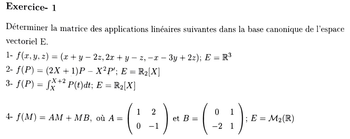
1) \(f(x,y,z)=(x+y-2z,\ 2x+y-z,\ -x-3y+2z)\), \(E=\mathbb R^3\)

Base canonique \((e_1,e_2,e_3)\) :

\[ f(1,0,0)=(1,2,-1),\quad f(0,1,0)=(1,1,-3),\quad f(0,0,1)=(-2,-1,2). \]

2) \(f(P)=(2X+1)P-X^2P'\), \(E=\mathbb R_2[X]\)

Base canonique \((1,X,X^2)\). On calcule, avec \(1'=0\), \(X'=1\), \((X^2)'=2X\) :

\[ \begin{aligned} f(1)&=(2X+1)\cdot1-0=1+2X &&\to(1,2,0),\\ f(X)&=(2X+1)X-X^2\cdot1=X+X^2 &&\to(0,1,1),\\ f(X^2)&=(2X+1)X^2-X^2\cdot2X=X^2 &&\to(0,0,1). \end{aligned} \]

On vérifie que \(f\) est bien à valeurs dans \(\mathbb R_2[X]\) : le terme en \(X^3\) de \(f(X^2)\) s'annule (\(2X^3-2X^3=0\)).

3) \(f(P)=\displaystyle\int_X^{X+2}P(t)\,dt\), \(E=\mathbb R_2[X]\)

Pour \(P=X^k\) : \(\displaystyle\int_X^{X+2}t^k\,dt=\dfrac{(X+2)^{k+1}-X^{k+1}}{k+1}\).

\[ \begin{aligned} f(1)&=(X+2)-X=2 &&\to(2,0,0),\\ f(X)&=\frac{(X+2)^2-X^2}{2}=\frac{4X+4}{2}=2X+2 &&\to(2,2,0),\\ f(X^2)&=\frac{(X+2)^3-X^3}{3}=\frac{6X^2+12X+8}{3}=2X^2+4X+\frac83 &&\to\left(\tfrac83,4,2\right). \end{aligned} \]

Matrice triangulaire supérieure : \(f\) conserve le degré (intégrer sur une longueur 2 ne change pas le degré).

4) \(f(M)=AM+MB\), \(A=\begin{pmatrix}1&2\\0&-1\end{pmatrix}\), \(B=\begin{pmatrix}0&1\\-2&1\end{pmatrix}\), \(E=\mathcal M_2(\mathbb R)\)

Base canonique \((E_{11},E_{12},E_{21},E_{22})\) de \(\mathcal M_2(\mathbb R)\) ; on repère une matrice \(\begin{pmatrix}a&b\\c&d\end{pmatrix}\) par ses coordonnées \((a,b,c,d)\).

\[ \begin{aligned} f(E_{11})&=AE_{11}+E_{11}B=\begin{pmatrix}1&0\\0&0\end{pmatrix}+\begin{pmatrix}0&1\\0&0\end{pmatrix}=\begin{pmatrix}1&1\\0&0\end{pmatrix}\to(1,1,0,0),\\ f(E_{12})&=\begin{pmatrix}0&1\\0&0\end{pmatrix}+\begin{pmatrix}-2&1\\0&0\end{pmatrix}=\begin{pmatrix}-2&2\\0&0\end{pmatrix}\to(-2,2,0,0). \end{aligned} \]

Détail de \(E_{21}\) : \(AE_{21}=\begin{pmatrix}1&2\\0&-1\end{pmatrix}\begin{pmatrix}0&0\\1&0\end{pmatrix}=\begin{pmatrix}2&0\\-1&0\end{pmatrix}\) et \(E_{21}B=\begin{pmatrix}0&0\\1&0\end{pmatrix}\begin{pmatrix}0&1\\-2&1\end{pmatrix}=\begin{pmatrix}0&0\\0&1\end{pmatrix}\), donc

\[ f(E_{21})=\begin{pmatrix}2&0\\-1&1\end{pmatrix}\to(2,0,-1,1). \]

Détail de \(E_{22}\) : \(AE_{22}=\begin{pmatrix}0&2\\0&-1\end{pmatrix}\) et \(E_{22}B=\begin{pmatrix}0&0\\-2&1\end{pmatrix}\), donc

\[ f(E_{22})=\begin{pmatrix}0&2\\-2&0\end{pmatrix}\to(0,2,-2,0). \]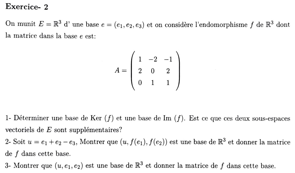

\(A=\begin{pmatrix}1&-2&-1\\2&0&2\\0&1&1\end{pmatrix}\), matrice de \(f\) dans la base \(e=(e_1,e_2,e_3)\).

1) Base de \(\operatorname{Ker}f\), base de \(\operatorname{Im}f\), supplémentaires ?

Noyau. \((x,y,z)\in\operatorname{Ker}f\iff A\begin{pmatrix}x\\y\\z\end{pmatrix}=0\) :

\[ \begin{cases}x-2y-z=0\\2x+2z=0\\y+z=0\end{cases} \iff\begin{cases}z=-x\\ y=-z=x\\ x-2x+x=0\ \checkmark\end{cases} \]

Donc \(\operatorname{Ker}f=\{(x,x,-x)\}=\operatorname{Vect}(u)\) avec \(u=(1,1,-1)=e_1+e_2-e_3\) (c'est le vecteur \(u\) de la question 2).

Image. \(\operatorname{Im}f=\operatorname{Vect}(f(e_1),f(e_2),f(e_3))\), colonnes de \(A\) : \(f(e_1)=(1,2,0)\), \(f(e_2)=(-2,0,1)\), \(f(e_3)=(-1,2,1)\). On remarque \(f(e_1)+f(e_2)=(-1,2,1)=f(e_3)\), donc \(f(e_3)\) est superflu. Les deux vecteurs \(f(e_1),f(e_2)\) ne sont pas colinéaires (\(0\) en 3ᵉ coordonnée pour le premier, \(1\) pour le second ; \(2\neq0\) en 2ᵉ pour le premier, \(0\) pour le second), donc ils forment une famille libre. Théorème du rang : \(\operatorname{rg}f=3-\dim\operatorname{Ker}f=3-1=2\) ✓.

Supplémentaires ? Il faut \(\operatorname{Ker}f\cap\operatorname{Im}f=\{0\}\) et \(\dim\operatorname{Ker}f+\dim\operatorname{Im}f=3\) (la 2ᵉ condition est vraie : \(1+2=3\)). Vérifions \(u\notin\operatorname{Im}f\) : si \(u=a f(e_1)+b f(e_2)\), alors 3ᵉ coordonnée : \(b=-1\) ; 2ᵉ : \(2a=1\), \(a=\tfrac12\) ; 1ʳᵉ : \(a-2b=\tfrac12+2=\tfrac52\neq1\) → contradiction. Donc \(u\notin\operatorname{Im}f\) ; comme \(\operatorname{Ker}f\) est la droite \(\operatorname{Vect}(u)\), l'intersection est \(\{0\}\).

2) \((u,f(e_1),f(e_2))\) est une base ; matrice de \(f\) dans cette base

Coordonnées dans \(e\) : \(u=(1,1,-1)\), \(f(e_1)=(1,2,0)\), \(f(e_2)=(-2,0,1)\). Matrice \(P=\begin{pmatrix}1&1&-2\\1&2&0\\-1&0&1\end{pmatrix}\). Son déterminant (développement selon la 3ᵉ ligne) :

\[ \det P=(-1)\begin{vmatrix}1&-2\\2&0\end{vmatrix}+1\cdot\begin{vmatrix}1&1\\1&2\end{vmatrix} =(-1)(0+4)+(2-1)=-4+1=-3\neq0. \]

(Cohérent avec la question 1 : \(u\) engendre le noyau, \(f(e_1),f(e_2)\) l'image, ces deux sous-espaces étant supplémentaires.) Donc \(\mathcal B_2=(u,f(e_1),f(e_2))\) est une base de \(\mathbb R^3\).

Images des vecteurs de \(\mathcal B_2\) :

• \(f(u)=0\) (car \(u\in\operatorname{Ker}f\)) → colonne \((0,0,0)\).
• \(f(f(e_1))=A\begin{pmatrix}1\\2\\0\end{pmatrix}=\begin{pmatrix}1-4\\2\\2\end{pmatrix}=\begin{pmatrix}-3\\2\\2\end{pmatrix}\). Or \(f(e_1)+2f(e_2)=(1,2,0)+(-4,0,2)=(-3,2,2)\). Donc \(f(f(e_1))=1\cdot f(e_1)+2\cdot f(e_2)\) → colonne \((0,1,2)\).
• \(f(f(e_2))=A\begin{pmatrix}-2\\0\\1\end{pmatrix}=\begin{pmatrix}-2-1\\-4+2\\1\end{pmatrix}=\begin{pmatrix}-3\\-2\\1\end{pmatrix}\). Or \(-f(e_1)+f(e_2)=(-1,-2,0)+(-2,0,1)=(-3,-2,1)\). Donc \(f(f(e_2))=-f(e_1)+f(e_2)\) → colonne \((0,-1,1)\).

3) \((u,e_1,e_2)\) est une base ; matrice de \(f\) dans cette base

Matrice des coordonnées : \(\begin{pmatrix}1&1&0\\1&0&1\\-1&0&0\end{pmatrix}\) (colonnes \(u,e_1,e_2\)). Développement selon la 3ᵉ ligne : \(\det=(-1)\begin{vmatrix}1&0\\0&1\end{vmatrix}=-1\neq0\) → base. Directement : \(e_3=e_1+e_2-u\), donc \(e_3\in\operatorname{Vect}(u,e_1,e_2)\) et la famille engendre \(\mathbb R^3\).

• \(f(u)=0\) → \((0,0,0)\).
• \(f(e_1)=(1,2,0)=e_1+2e_2\) → \((0,1,2)\).
• \(f(e_2)=(-2,0,1)=-2e_1+e_3=-2e_1+(e_1+e_2-u)=-u-e_1+e_2\) → \((-1,-1,1)\).

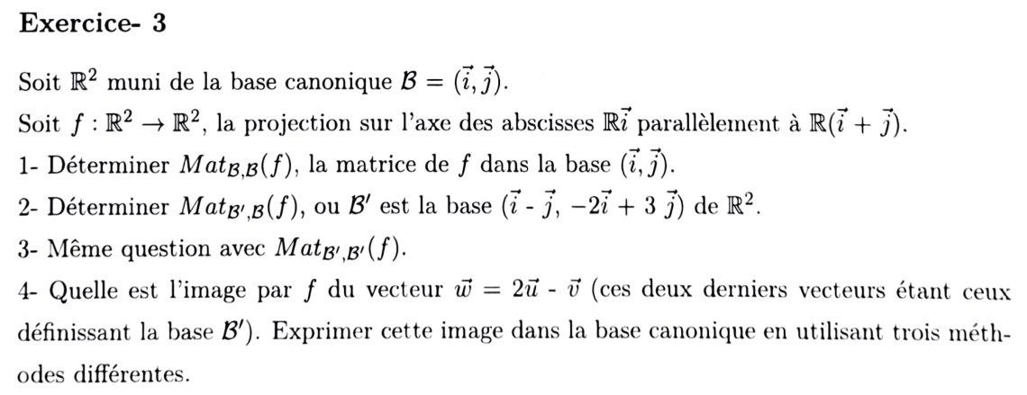
1) \(\operatorname{Mat}_{\mathcal B,\mathcal B}(f)\)

\(f\) est la projection sur \(\mathbb R\vec\imath\) parallèlement à \(\mathbb R(\vec\imath+\vec\jmath)\) : \(f(\vec\imath)=\vec\imath\) (vecteur de l'axe, fixé) et \(f(\vec\imath+\vec\jmath)=\vec0\) (vecteur de la direction). Donc

\[ f(\vec\jmath)=f\big((\vec\imath+\vec\jmath)-\vec\imath\big)=\vec0-\vec\imath=-\vec\imath. \]

Vérification : \(f(1,1)=(0,0)\) ✓, \(f(x,0)=(x,0)\) ✓.

2) \(\operatorname{Mat}_{\mathcal B',\mathcal B}(f)\), \(\mathcal B'=(\vec\imath-\vec\jmath,\,-2\vec\imath+3\vec\jmath)\)

On note \(b_1'=\vec\imath-\vec\jmath=(1,-1)\), \(b_2'=-2\vec\imath+3\vec\jmath=(-2,3)\). (\(\mathcal B'\) est une base : \(\det\begin{pmatrix}1&-2\\-1&3\end{pmatrix}=3-2=1\neq0\).)

\[ f(b_1')=f(1,-1)=(1-(-1),0)=(2,0)=2\vec\imath,\qquad f(b_2')=f(-2,3)=(-2-3,0)=(-5,0)=-5\vec\imath. \]

On exprime dans la base d'arrivée \(\mathcal B\) (canonique) :

Contrôle du produit : \(\begin{pmatrix}1&-1\\0&0\end{pmatrix}\begin{pmatrix}1&-2\\-1&3\end{pmatrix}=\begin{pmatrix}2&-5\\0&0\end{pmatrix}\) ✓.

3) \(\operatorname{Mat}_{\mathcal B'}(f)=\operatorname{Mat}_{\mathcal B',\mathcal B'}(f)\)

Il faut maintenant exprimer \(f(b_1')=2\vec\imath\) et \(f(b_2')=-5\vec\imath\) dans la base \(\mathcal B'\). On inverse : \(P^{-1}=\dfrac1{\det P}\begin{pmatrix}3&2\\1&1\end{pmatrix}=\begin{pmatrix}3&2\\1&1\end{pmatrix}\) (formule \(\frac1{ad-bc}\begin{pmatrix}d&-b\\-c&a\end{pmatrix}\)). Les colonnes de \(P^{-1}\) donnent \(\vec\imath=3b_1'+b_2'\) et \(\vec\jmath=2b_1'+b_2'\). Vérification : \(3(1,-1)+(-2,3)=(1,0)\) ✓ et \(2(1,-1)+(-2,3)=(0,1)\) ✓. Donc

\[ f(b_1')=2\vec\imath=6b_1'+2b_2',\qquad f(b_2')=-5\vec\imath=-15b_1'-5b_2'. \]

Contrôle : \(P^{-1}\begin{pmatrix}2&-5\\0&0\end{pmatrix}=\begin{pmatrix}3\cdot2&3\cdot(-5)\\1\cdot2&1\cdot(-5)\end{pmatrix}=\begin{pmatrix}6&-15\\2&-5\end{pmatrix}\) ✓. Autre contrôle : \(\operatorname{tr}=6-5=1=\operatorname{tr}\begin{pmatrix}1&-1\\0&0\end{pmatrix}\) et \(\det=-30+30=0\) (la trace et le déterminant ne changent pas par changement de base) ✓.

4) Image de \(\vec w=2\vec u-\vec v\) (avec \(\vec u=b_1'\), \(\vec v=b_2'\)) — trois méthodes

Coordonnées de \(\vec w\) dans \(\mathcal B'\) : \((2,-1)\). Dans la base canonique : \(\vec w=2(1,-1)-(-2,3)=(4,-5)\).

Méthode 1 — par la matrice canonique. \(f(\vec w)=\begin{pmatrix}1&-1\\0&0\end{pmatrix}\begin{pmatrix}4\\-5\end{pmatrix}=\begin{pmatrix}4+5\\0\end{pmatrix}=\begin{pmatrix}9\\0\end{pmatrix}\).

Méthode 2 — par \(\operatorname{Mat}_{\mathcal B',\mathcal B}(f)\) (départ \(\mathcal B'\), arrivée canonique : on lui donne directement les coordonnées dans \(\mathcal B'\) et on obtient le résultat dans la base canonique) : \(\begin{pmatrix}2&-5\\0&0\end{pmatrix}\begin{pmatrix}2\\-1\end{pmatrix}=\begin{pmatrix}4+5\\0\end{pmatrix}=\begin{pmatrix}9\\0\end{pmatrix}\).

Méthode 3 — par \(\operatorname{Mat}_{\mathcal B'}(f)\) (résultat dans \(\mathcal B'\), puis conversion) : \(\begin{pmatrix}6&-15\\2&-5\end{pmatrix}\begin{pmatrix}2\\-1\end{pmatrix}=\begin{pmatrix}12+15\\4+5\end{pmatrix}=\begin{pmatrix}27\\9\end{pmatrix}_{\mathcal B'}\), soit \(f(\vec w)=27b_1'+9b_2'=27(1,-1)+9(-2,3)=(27-18,\,-27+27)=(9,0)\).

Méthode 4 (contrôle) — par linéarité. \(f(\vec w)=2f(\vec u)-f(\vec v)=2(2,0)-(-5,0)=(9,0)\).

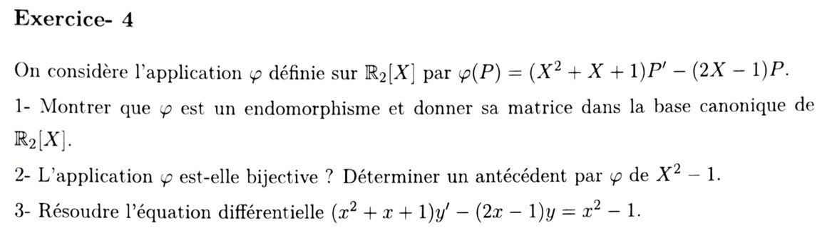
1) \(\varphi\) est un endomorphisme ; matrice dans la base canonique

Linéarité. Pour \(P,Q\in\mathbb R_2[X]\) et \(\lambda\in\mathbb R\) : la dérivation est linéaire, donc \(\varphi(\lambda P+Q)=(X^2+X+1)(\lambda P'+Q')-(2X-1)(\lambda P+Q)=\lambda\varphi(P)+\varphi(Q)\).

À valeurs dans \(\mathbb R_2[X]\). Pour \(P=aX^2+bX+c\) : \(P'=2aX+b\) et

\[ \varphi(P)=(X^2+X+1)(2aX+b)-(2X-1)(aX^2+bX+c). \]

Le terme en \(X^3\) vaut \(2a-2a=0\) : \(\deg\varphi(P)\le2\). Donc \(\varphi\in\mathcal L(\mathbb R_2[X])\) : endomorphisme. Matrice dans \((1,X,X^2)\) :

\[ \begin{aligned} \varphi(1)&=-(2X-1)=1-2X &&\to(1,-2,0),\\ \varphi(X)&=(X^2+X+1)-(2X-1)X=X^2+X+1-2X^2+X=-X^2+2X+1 &&\to(1,2,-1),\\ \varphi(X^2)&=(X^2+X+1)\,2X-(2X-1)X^2=2X^3+2X^2+2X-2X^3+X^2=3X^2+2X &&\to(0,2,3). \end{aligned} \]

2) \(\varphi\) bijective ? Antécédent de \(X^2-1\)

Développement du déterminant selon la 1ʳᵉ ligne :

\[ \det M=1\begin{vmatrix}2&2\\-1&3\end{vmatrix}-1\begin{vmatrix}-2&2\\0&3\end{vmatrix}+0 =1\cdot(6+2)-1\cdot(-6-0)=8+6=14\neq0. \]

\(M\) est inversible, donc \(\varphi\) est bijective (endomorphisme d'un espace de dimension finie de matrice inversible).

Antécédent de \(X^2-1\), de coordonnées \((-1,0,1)\) : on résout \(M\begin{pmatrix}c\\b\\a\end{pmatrix}=\begin{pmatrix}-1\\0\\1\end{pmatrix}\) pour \(P=aX^2+bX+c\) :

\[ \begin{cases}c+b=-1\\-2c+2b+2a=0\\-b+3a=1\end{cases} \]

(1) donne \(c=-1-b\). (2) : \(2+2b+2b+2a=0\), soit \(a=-1-2b\). (3) : \(-b+3(-1-2b)=1\), soit \(-7b=4\), \(b=-\tfrac47\). Alors \(a=-1+\tfrac87=\tfrac17\) et \(c=-1+\tfrac47=-\tfrac37\).

Vérification : \(\varphi(P_0)=\frac17\big[(X^2+X+1)(2X-4)-(2X-1)(X^2-4X-3)\big]\). Premier produit : \(2X^3-4X^2+2X^2-4X+2X-4=2X^3-2X^2-2X-4\). Second : \(2X^3-8X^2-6X-X^2+4X+3=2X^3-9X^2-2X+3\). Différence : \(7X^2-7\). Donc \(\varphi(P_0)=X^2-1\) ✓.

3) Résoudre \((x^2+x+1)y'-(2x-1)y=x^2-1\)

L'équation s'écrit \(\varphi(y)=x^2-1\) où \(\varphi\) agit maintenant sur des fonctions dérivables (sur \(\mathbb R\), car \(x^2+x+1>0\) : discriminant \(1-4=-3<0\)). C'est une équation différentielle linéaire du 1ᵉʳ ordre : solution générale = solution particulière + solution générale de l'équation homogène.

Solution particulière : le polynôme \(P_0\) de la question 2 (c'est précisément le but de la question).

Équation homogène \((x^2+x+1)y'=(2x-1)y\), soit \(\dfrac{y'}{y}=\dfrac{2x-1}{x^2+x+1}\). On décompose \(2x-1=(2x+1)-2\) (car \((x^2+x+1)'=2x+1\)) :

\[ \int\frac{2x-1}{x^2+x+1}\,dx=\ln(x^2+x+1)-2\int\frac{dx}{x^2+x+1}. \]

Forme canonique \(x^2+x+1=\big(x+\tfrac12\big)^2+\tfrac34\), donc \(\displaystyle\int\frac{dx}{x^2+x+1}=\frac{2}{\sqrt3}\arctan\!\Big(\frac{2x+1}{\sqrt3}\Big)\). D'où

\[ y_h(x)=C\,(x^2+x+1)\exp\!\Big(-\frac{4}{\sqrt3}\arctan\frac{2x+1}{\sqrt3}\Big),\quad C\in\mathbb R. \]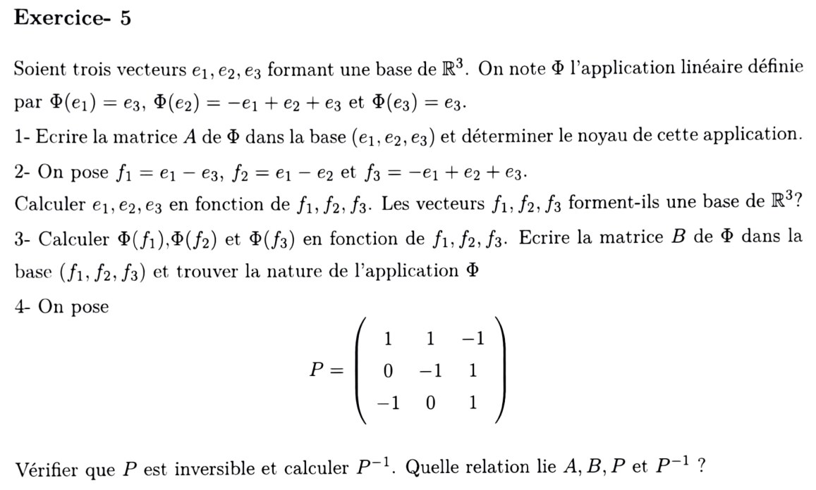

1) Matrice \(A\) de \(\Phi\) dans \((e_1,e_2,e_3)\) et noyau

Colonnes = images : \(\Phi(e_1)=e_3=(0,0,1)\), \(\Phi(e_2)=-e_1+e_2+e_3=(-1,1,1)\), \(\Phi(e_3)=e_3=(0,0,1)\).

Noyau : \(A\begin{pmatrix}x\\y\\z\end{pmatrix}=\begin{pmatrix}-y\\y\\x+y+z\end{pmatrix}=0\iff y=0,\ z=-x\). Donc \(\ker\Phi=\{(x,0,-x)\}=\operatorname{Vect}(e_1-e_3)\) (droite ; \(\operatorname{rg}\Phi=3-1=2\)).

2) \(f_1=e_1-e_3,\ f_2=e_1-e_2,\ f_3=-e_1+e_2+e_3\) : \(e_i\) en fonction des \(f_j\) ; base ?

On remarque \(f_2+f_3=(e_1-e_2)+(-e_1+e_2+e_3)=e_3\). Puis \(f_1+e_3=e_1\), donc \(e_1=f_1+f_2+f_3\). Enfin \(e_2=e_1-f_2=f_1+f_2+f_3-f_2=f_1+f_3\).

Vérification : \(f_1+f_2+f_3=(1+1-1,\,0-1+1,\,-1+0+1)=(1,0,0)=e_1\) ✓. Les trois \(e_i\) sont combinaisons linéaires de \(f_1,f_2,f_3\), donc \(\operatorname{Vect}(f_1,f_2,f_3)=\mathbb R^3\) : famille génératrice de 3 vecteurs dans un espace de dimension 3, c'est une base.

3) \(\Phi(f_j)\) ; matrice \(B\) dans \((f_1,f_2,f_3)\) ; nature de \(\Phi\)

\[ \begin{aligned} \Phi(f_1)&=\Phi(e_1)-\Phi(e_3)=e_3-e_3=0,\\ \Phi(f_2)&=\Phi(e_1)-\Phi(e_2)=e_3-(-e_1+e_2+e_3)=e_1-e_2=f_2,\\ \Phi(f_3)&=-\Phi(e_1)+\Phi(e_2)+\Phi(e_3)=-e_3+(-e_1+e_2+e_3)+e_3=-e_1+e_2+e_3=f_3. \end{aligned} \]

(On vérifie \(\Phi\circ\Phi=\Phi\) : \(B^2=B\), caractéristique d'un projecteur.)

4) \(P\) inversible, \(P^{-1}\), relation entre \(A,B,P,P^{-1}\)

\(P=\begin{pmatrix}1&1&-1\\0&-1&1\\-1&0&1\end{pmatrix}\) a pour colonnes les coordonnées de \(f_1,f_2,f_3\) dans \((e_1,e_2,e_3)\) : c'est la matrice de passage de \((e)\) vers \((f)\). Déterminant (développement selon la 1ʳᵉ colonne) : \(\det P=1\begin{vmatrix}-1&1\\0&1\end{vmatrix}+(-1)\begin{vmatrix}1&-1\\-1&1\end{vmatrix} =1\cdot(-1)-(1-1)=-1\neq0\). Donc \(P\) est inversible. D'après la question 2, les colonnes de \(P^{-1}\) donnent \(e_1,e_2,e_3\) dans la base \((f)\) :

Vérification de \(PP^{-1}=I_3\) : 1ʳᵉ ligne de \(P\), \((1,1,-1)\), contre les colonnes \((1,1,1)\), \((1,0,1)\), \((0,1,1)\) : \(1+1-1=1\), \(1+0-1=0\), \(0+1-1=0\) ✓ ; 2ᵉ ligne \((0,-1,1)\) : \(-1+1=0\), \(0+1=1\), \(-1+1=0\) ✓ ; 3ᵉ ligne \((-1,0,1)\) : \(-1+1=0\), \(-1+1=0\), \(1\) ✓.

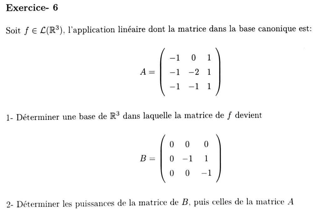
\(A=\begin{pmatrix}-1&0&1\\-1&-2&1\\-1&-1&1\end{pmatrix}\), \(B=\begin{pmatrix}0&0&0\\0&-1&1\\0&0&-1\end{pmatrix}\).

1) Base \((b_1,b_2,b_3)\) dans laquelle la matrice de \(f\) est \(B\)

\(b_1\) : \(Av=0\iff\begin{cases}-x+z=0\\-x-2y+z=0\\-x-y+z=0\end{cases}\). (1) : \(z=x\) ; (2) : \(-2y=0\), \(y=0\) ; (3) : \(-x-0+x=0\) ✓. On prend \(b_1=(1,0,1)\).

\(b_2\) : \((A+I)v=0\) avec \(A+I=\begin{pmatrix}0&0&1\\-1&-1&1\\-1&-1&2\end{pmatrix}\) : (1) \(z=0\) ; (2) \(-x-y=0\) ; (3) \(-x-y+2z=0\) ✓. On prend \(b_2=(1,-1,0)\).

\(b_3\) : \((A+I)b_3=b_2\) : \(\begin{cases}z=1\\-x-y+z=-1\\-x-y+2z=0\end{cases}\) : \(z=1\), puis \(x+y=2\) (équation 2) et l'équation 3 donne \(-x-y+2=0\) ✓ (cohérent). On prend \(b_3=(2,0,1)\).

Vérifications. \(Ab_1=(-1+1,\,-1+1,\,-1+1)=0\) ✓. \(Ab_2=(-1,\,-1+2,\,-1+1)=(-1,1,0)=-b_2\) ✓. \(Ab_3=(-2+1,\,-2+1,\,-2+1)=(-1,-1,-1)\) et \(b_2-b_3=(1-2,\,-1-0,\,0-1)=(-1,-1,-1)\) ✓.

C'est une base : \(P=\begin{pmatrix}1&1&2\\0&-1&0\\1&0&1\end{pmatrix}\) (colonnes \(b_1,b_2,b_3\)), \(\det P=(-1)\cdot(-1)^{2+2}\begin{vmatrix}1&2\\1&1\end{vmatrix}=(-1)(1-2)=1\neq0\).

2) Puissances de \(B\), puis de \(A\)

Puissances de \(B\). \(B\) est diagonale par blocs : le bloc \(1\times1\) vaut \(0\) et le bloc \(T=\begin{pmatrix}-1&1\\0&-1\end{pmatrix}=-I_2+N\) avec \(N=\begin{pmatrix}0&1\\0&0\end{pmatrix}\), \(N^2=0\). Comme \(-I_2\) et \(N\) commutent, le binôme de Newton s'applique et tous les termes en \(N^k\), \(k\ge2\), disparaissent :

\[ T^n=(-I_2+N)^n=(-1)^nI_2+n(-1)^{n-1}N=\begin{pmatrix}(-1)^n&n(-1)^{n-1}\\0&(-1)^n\end{pmatrix}. \]

Puissances de \(A\). \(A^n=PB^nP^{-1}\) avec \(P^{-1}=\begin{pmatrix}-1&-1&2\\0&-1&0\\1&1&-1\end{pmatrix}\) (on vérifie \(PP^{-1}\) : 1ʳᵉ ligne de \(P\), \((1,1,2)\), contre les colonnes de \(P^{-1}\) : \(-1+0+2=1\), \(-1-1+2=0\), \(2+0-2=0\) ✓ ; 2ᵉ ligne \((0,-1,0)\) : \(0\), \(1\), \(0\) ✓ ; 3ᵉ ligne \((1,0,1)\) : \(-1+1=0\), \(-1+1=0\), \(2-1=1\) ✓). Posons \(s=(-1)^n\), donc \(n(-1)^{n-1}=-ns\) :

\[ PB^n=\begin{pmatrix}1&1&2\\0&-1&0\\1&0&1\end{pmatrix}\begin{pmatrix}0&0&0\\0&s&-ns\\0&0&s\end{pmatrix} =\begin{pmatrix}0&s&(2-n)s\\0&-s&ns\\0&0&s\end{pmatrix}, \] \[ A^n=PB^nP^{-1}=\begin{pmatrix}0&s&(2-n)s\\0&-s&ns\\0&0&s\end{pmatrix}\begin{pmatrix}-1&-1&2\\0&-1&0\\1&1&-1\end{pmatrix} =s\begin{pmatrix}2-n&1-n&n-2\\n&n+1&-n\\1&1&-1\end{pmatrix}. \]

Contrôle : \(n=1\) donne \(-\begin{pmatrix}1&0&-1\\1&2&-1\\1&1&-1\end{pmatrix}=A\) ✓ ; \(n=2\) donne \(\begin{pmatrix}0&-1&0\\2&3&-2\\1&1&-1\end{pmatrix}=A^2\) (calcul direct de \(A\cdot A\), 1ʳᵉ ligne : \((-1,0,1)\cdot\)colonnes de \(A\) = \((1-1,\,0+0-1,\,-1+0+1)=(0,-1,0)\) ✓).

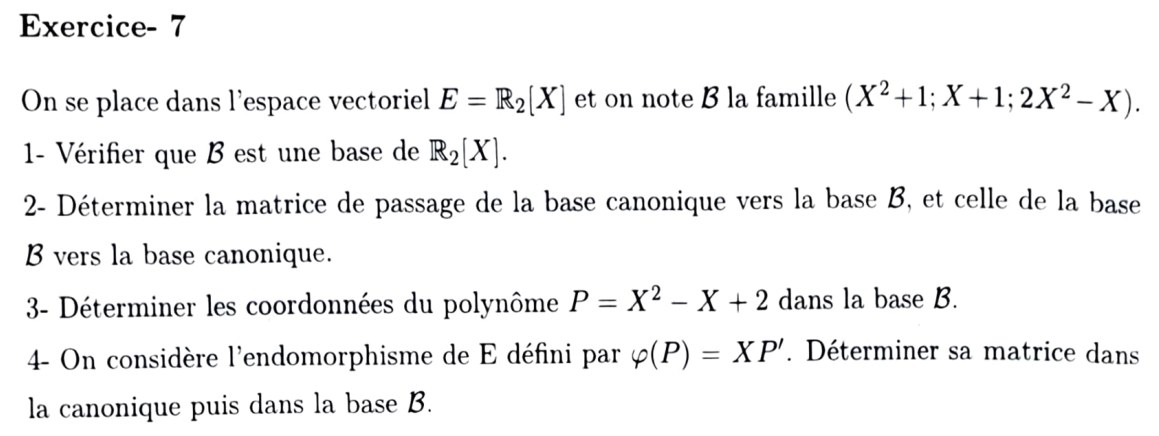
1) \(\mathcal B=(X^2+1,\ X+1,\ 2X^2-X)\) est une base de \(\mathbb R_2[X]\)

Dans la base canonique \((1,X,X^2)\) (coordonnées dans l'ordre \(1,X,X^2\)) : \(X^2+1\to(1,0,1)\), \(X+1\to(1,1,0)\), \(2X^2-X\to(0,-1,2)\). Matrice des coordonnées \(P=\begin{pmatrix}1&1&0\\0&1&-1\\1&0&2\end{pmatrix}\) :

\[ \det P=1\begin{vmatrix}1&-1\\0&2\end{vmatrix}-1\begin{vmatrix}0&-1\\1&2\end{vmatrix}+0=2-(0+1)=1\neq0. \]

2) Matrices de passage canonique → \(\mathcal B\) et \(\mathcal B\) → canonique

Par définition (colonnes = coordonnées de la nouvelle base dans l'ancienne) :

\[ P_{\text{can}\to\mathcal B}=P=\begin{pmatrix}1&1&0\\0&1&-1\\1&0&2\end{pmatrix}. \]

La matrice de passage inverse est \(P^{-1}\). Calcul par la comatrice (\(\det P=1\)) : on obtient

\[ P_{\mathcal B\to\text{can}}=P^{-1}=\begin{pmatrix}2&-2&-1\\-1&2&1\\-1&1&1\end{pmatrix}. \]

Vérification de \(PP^{-1}=I_3\) : 1ʳᵉ ligne de \(P\), \((1,1,0)\), contre les colonnes \((2,-1,-1)\), \((-2,2,1)\), \((-1,1,1)\) : \(2-1=1\), \(-2+2=0\), \(-1+1=0\) ✓ ; 2ᵉ ligne \((0,1,-1)\) : \(-1+1=0\), \(2-1=1\), \(1-1=0\) ✓ ; 3ᵉ ligne \((1,0,2)\) : \(2-2=0\), \(-2+2=0\), \(-1+2=1\) ✓.

Interprétation : les colonnes de \(P^{-1}\) expriment \(1,X,X^2\) dans \(\mathcal B\). Exemple : \(1=2(X^2+1)-(X+1)-(2X^2-X)\) (développé : \(2X^2+2-X-1-2X^2+X=1\) ✓).

3) Coordonnées de \(P=X^2-X+2\) dans \(\mathcal B\)

Coordonnées canoniques : \((2,-1,1)\). Dans \(\mathcal B\) : \(X_{\mathcal B}=P^{-1}X_{\text{can}}\) :

\[ \begin{pmatrix}2&-2&-1\\-1&2&1\\-1&1&1\end{pmatrix}\begin{pmatrix}2\\-1\\1\end{pmatrix} =\begin{pmatrix}4+2-1\\-2-2+1\\-2-1+1\end{pmatrix}=\begin{pmatrix}5\\-3\\-2\end{pmatrix}. \]

Vérification : \(5X^2+5-3X-3-4X^2+2X=X^2-X+2\) ✓.

4) \(\varphi(P)=XP'\) : matrice dans la canonique puis dans \(\mathcal B\)

\(\varphi(1)=0\), \(\varphi(X)=X\cdot1=X\), \(\varphi(X^2)=X\cdot2X=2X^2\) (\(\varphi\) est bien un endomorphisme de \(\mathbb R_2[X]\)).

Dans la base \(\mathcal B\) : \(\operatorname{Mat}_{\mathcal B}(\varphi)=P^{-1}DP\). D'abord \(DP=\begin{pmatrix}0&0&0\\0&1&-1\\2&0&4\end{pmatrix}\) (chaque ligne de \(P\) multipliée par le coefficient diagonal correspondant), puis

\[ P^{-1}(DP)=\begin{pmatrix}2&-2&-1\\-1&2&1\\-1&1&1\end{pmatrix}\begin{pmatrix}0&0&0\\0&1&-1\\2&0&4\end{pmatrix} =\begin{pmatrix}-2&-2&-2\\2&2&2\\2&1&3\end{pmatrix}. \]

Vérification sur la 1ʳᵉ colonne : \(\varphi(X^2+1)=X\cdot2X=2X^2\), dont les coordonnées dans \(\mathcal B\) sont \(P^{-1}(0,0,2)=(-2,2,2)\) ✓ (colonne 1). Trace conservée : \(-2+2+3=3=0+1+2\) ✓.

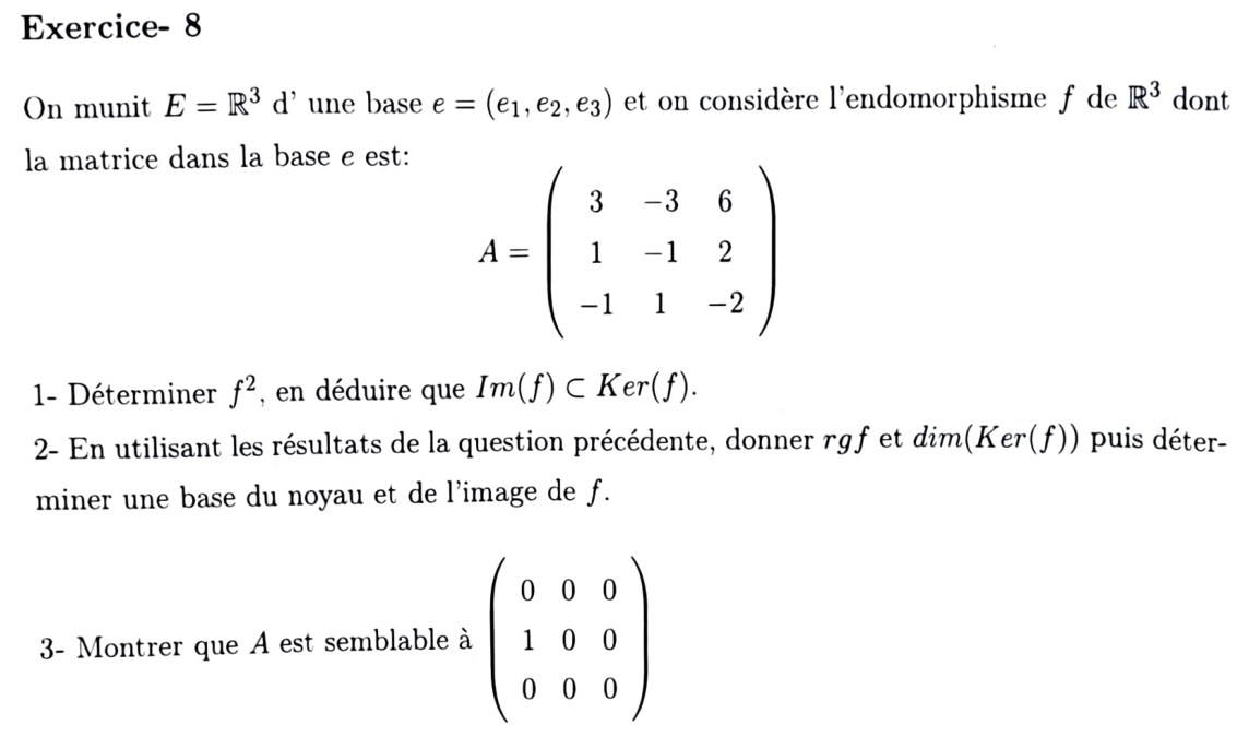
\(A=\begin{pmatrix}3&-3&6\\1&-1&2\\-1&1&-2\end{pmatrix}\).

1) Calcul de \(f^2\) ; \(\operatorname{Im}f\subset\operatorname{Ker}f\)

Produit \(A\times A\) (ligne × colonne). Colonnes de \(A\) : \(c_1=(3,1,-1)\), \(c_2=(-3,-1,1)\), \(c_3=(6,2,-2)\).

\[ \begin{aligned} &\text{Ligne }(3,-3,6):\ 9-3-6=0,\ \ -9+3+6=0,\ \ 18-6-12=0;\\ &\text{Ligne }(1,-1,2):\ 3-1-2=0,\ \ -3+1+2=0,\ \ 6-2-4=0;\\ &\text{Ligne }(-1,1,-2):\ -3+1+2=0,\ \ 3-1-2=0,\ \ -6+2+4=0. \end{aligned} \]

Inclusion : soit \(y\in\operatorname{Im}f\), \(y=f(x)\). Alors \(f(y)=f(f(x))=f^2(x)=0\), donc \(y\in\operatorname{Ker}f\).

2) \(\operatorname{rg}f\), \(\dim\operatorname{Ker}f\), bases du noyau et de l'image

On a \(c_2=-c_1\) et \(c_3=2c_1\) avec \(c_1\neq0\) : \(\operatorname{Im}f=\operatorname{Vect}(c_1)\), donc \(\operatorname{rg}f=1\). Théorème du rang : \(\dim\operatorname{Ker}f=3-1=2\). (Cohérent avec la question 1 : \(\dim\operatorname{Im}f=1\le\dim\operatorname{Ker}f=2\).)

Noyau : les trois lignes sont proportionnelles à \((1,-1,2)\) (\((3,-3,6)=3\cdot(1,-1,2)\), \((-1,1,-2)=-(1,-1,2)\)), donc \(\operatorname{Ker}f\) est le plan d'équation \(x-y+2z=0\) : \((x,y,z)=y(1,1,0)+z(-2,0,1)\). Base : \(\big((1,1,0),(-2,0,1)\big)\). On vérifie \(c_1=(3,1,-1)\in\operatorname{Ker}f\) : \(3-1-2=0\) ✓ (en effet \(c_1=(1,1,0)-(-2,0,1)=(3,1,-1)\), combinaison des deux vecteurs de base).

3) \(A\) est semblable à \(\begin{pmatrix}0&0&0\\1&0&0\\0&0&0\end{pmatrix}\)

On prend \(b_1=e_1=(1,0,0)\) (\(f(e_1)\neq0\)), \(b_2=f(b_1)=(3,1,-1)\) (dans \(\operatorname{Ker}f\) car \(\operatorname{Im}f\subset\operatorname{Ker}f\), donc \(f(b_2)=0\)), et \(b_3=(1,1,0)\in\operatorname{Ker}f\), non colinéaire à \(b_2\) (\(b_2\) et \(b_3\) sont donc deux vecteurs indépendants du plan \(\operatorname{Ker}f\)).

Base ? \(Q=\begin{pmatrix}1&3&1\\0&1&1\\0&-1&0\end{pmatrix}\) (colonnes \(b_1,b_2,b_3\)) : \(\det Q=1\begin{vmatrix}1&1\\-1&0\end{vmatrix}=1\cdot(0+1)=1\neq0\) ✓.

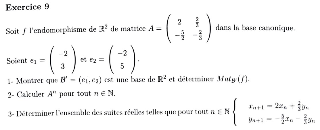
\(A=\begin{pmatrix}2&\tfrac23\\-\tfrac52&-\tfrac23\end{pmatrix}\), \(e_1=\begin{pmatrix}-2\\3\end{pmatrix}\), \(e_2=\begin{pmatrix}-2\\5\end{pmatrix}\).

1) \(\mathcal B'=(e_1,e_2)\) est une base de \(\mathbb R^2\) ; \(\operatorname{Mat}_{\mathcal B'}(f)\)

\(P=\begin{pmatrix}-2&-2\\3&5\end{pmatrix}\), \(\det P=(-2)(5)-(-2)(3)=-10+6=-4\neq0\) : \(e_1,e_2\) indépendants, donc base de \(\mathbb R^2\) (dimension 2).

Images : \(f(e_1)=Ae_1=\begin{pmatrix}2(-2)+\frac23\cdot3\\-\frac52(-2)-\frac23\cdot3\end{pmatrix}=\begin{pmatrix}-4+2\\5-2\end{pmatrix}=\begin{pmatrix}-2\\3\end{pmatrix}=e_1\) ; \(f(e_2)=Ae_2=\begin{pmatrix}-4+\frac{10}3\\5-\frac{10}3\end{pmatrix}=\begin{pmatrix}-\frac23\\\frac53\end{pmatrix}=\tfrac13\begin{pmatrix}-2\\5\end{pmatrix}=\tfrac13e_2\).

2) \(A^n\) pour tout \(n\in\mathbb N\)

\(A=PDP^{-1}\), donc \(A^n=PD^nP^{-1}\) avec \(D^n=\begin{pmatrix}1&0\\0&3^{-n}\end{pmatrix}\) (valable aussi pour \(n=0\)). \(P^{-1}=\dfrac1{-4}\begin{pmatrix}5&2\\-3&-2\end{pmatrix}=\begin{pmatrix}-\frac54&-\frac12\\\frac34&\frac12\end{pmatrix}\) (formule \(\frac1{ad-bc}\begin{pmatrix}d&-b\\-c&a\end{pmatrix}\)). Posons \(r=3^{-n}\) :

\[ PD^n=\begin{pmatrix}-2&-2r\\3&5r\end{pmatrix},\qquad A^n=\begin{pmatrix}-2&-2r\\3&5r\end{pmatrix}\begin{pmatrix}-\frac54&-\frac12\\\frac34&\frac12\end{pmatrix} =\begin{pmatrix}\frac52-\frac32r&1-r\\-\frac{15}4+\frac{15}4r&-\frac32+\frac52r\end{pmatrix}. \]

Contrôles : \(n=0\) (\(r=1\)) : \(A^0=I_2\) ✓. \(n=1\) (\(r=\frac13\)) : \(\begin{pmatrix}\frac52-\frac12&\frac23\\-\frac{15}4+\frac54&-\frac32+\frac56\end{pmatrix}=\begin{pmatrix}2&\frac23\\-\frac52&-\frac23\end{pmatrix}=A\) ✓. Limite : \(A^n\to\begin{pmatrix}\frac52&1\\-\frac{15}4&-\frac32\end{pmatrix}\) (projecteur sur \(\operatorname{Vect}(e_1)\) parallèlement à \(\operatorname{Vect}(e_2)\)).

3) Suites réelles telles que \(\begin{cases}x_{n+1}=2x_n+\frac23y_n\\y_{n+1}=-\frac52x_n-\frac23y_n\end{cases}\)

En posant \(X_n=\begin{pmatrix}x_n\\y_n\end{pmatrix}\) : \(X_{n+1}=AX_n\), donc \(X_n=A^nX_0\) (récurrence immédiate), avec \(X_0=(x_0,y_0)\in\mathbb R^2\) quelconque. Les suites solutions sont donc en bijection avec les conditions initiales \((x_0,y_0)\in\mathbb R^2\).

Forme explicite en développant \(A^nX_0\) :

\[ x_n=\Big(\tfrac52x_0+y_0\Big)-\Big(\tfrac32x_0+y_0\Big)3^{-n},\qquad y_n=-\Big(\tfrac{15}4x_0+\tfrac32y_0\Big)+\Big(\tfrac{15}4x_0+\tfrac52y_0\Big)3^{-n}. \]

Forme géométrique plus parlante : décomposer \(X_0=a\,e_1+b\,e_2\) (\((a,b)\) coordonnées de \(X_0\) dans \(\mathcal B'\)). Comme \(f(e_1)=e_1\) et \(f(e_2)=\tfrac13e_2\), on a \(X_n=a\,e_1+b\,3^{-n}e_2\) :

Vérification : \(X_{n+1}=AX_n=a\,Ae_1+b\,3^{-n}Ae_2=a\,e_1+b\,3^{-n}\cdot\tfrac13e_2=a\,e_1+b\,3^{-(n+1)}e_2\) ✓.